Heat transfer solver on distributed domains

Case study 2: solving the Heat transfer problem

For a tightly coupled parallel calculation, consider a heat diffusion problem:

• we have a square metallic plate initially at 25 degrees (initial condition)
• we want to simulate the evolution of the temperature across the plate; governed by the 2D heat (diffusion) equation:
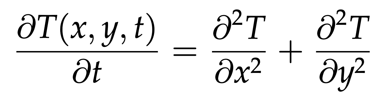
• discretize the solution \(T(x,y,t)\approx T^{(n)}_{i,j}\) with \(i=1,...,{\rm rows}\) and \(j=1,...,{\rm cols}\)
  • the upper left corner is (1,1) and the lower right corner is (rows,cols)
• the plate’s border is in contact with a different temperature distribution (boundary condition):
  • upper side \(T^{(n)}_{0,1..{\rm cols}}\equiv 0\)
  • left side \(T^{(n)}_{1..{\rm rows},0}\equiv 0\)
  • bottom side \(T^{(n)}_{{\rm rows}+1,1..{\rm cols}} = {80\cdot j/\rm cols}\) (linearly increasing from 0 to 80 degrees)
  • right side \(T^{(n)}_{1..{\rm rows},{\rm cols}+1} = 80\cdot i/{\rm rows}\) (linearly increasing from 0 to 80 degrees)

We discretize the equation with forward Euler time stepping:

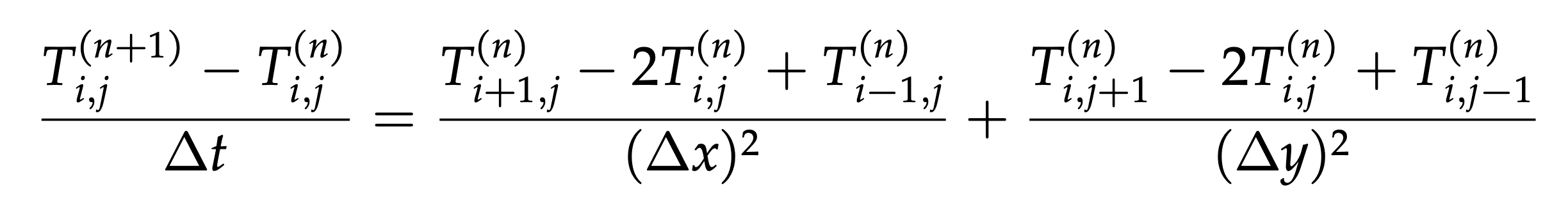
If for simplicity we assume \(\Delta x=\Delta y=1\) and \(\Delta t=1/4\), our finite difference equation becomes:

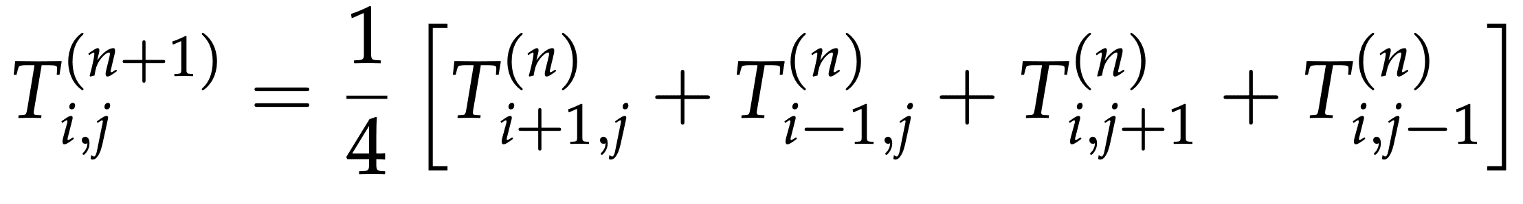
At each time iteration, at each point we’ll be computing the new temperature Tnew according to:

Tnew[i,j] = 0.25 * (T[i-1,j] + T[i+1,j] + T[i,j-1] + T[i,j+1])

• Tnew = new temperature computed at the current iteration
• T = temperature calculated at the past iteration (or the initial conditions at the first iteration)
• the indices (i,j) indicate the grid point located at the i-th row and the j-th column

Here is a serial implementation of this solver baseSolver.chpl:

use Time;
config const rows, cols = 100;   // number of rows and columns in our matrix
config const niter = 500;        // max number of iterations
config const tolerance = 1e-4: real;   // temperature difference tolerance
var count = 0: int;                    // the iteration counter
var delta: real;   // the greatest temperature difference between Tnew and T
var tmp: real;     // for temporary results

var T: [0..rows+1,0..cols+1] real;
var Tnew: [0..rows+1,0..cols+1] real;
T[1..rows,1..cols] = 25;

delta = tolerance*10;    // some safe initial large value
var watch: stopwatch;
watch.start();
while (count < niter && delta >= tolerance) {
  for i in 1..rows do T[i,cols+1] = 80.0*i/rows;   // right side boundary condition
  for j in 1..cols do T[rows+1,j] = 80.0*j/cols;   // bottom side boundary condition
  count += 1;    // update the iteration counter
  for i in 1..rows {
    for j in 1..cols {
      Tnew[i,j] = 0.25 * (T[i-1,j] + T[i+1,j] + T[i,j-1] + T[i,j+1]);
    }
  }
  delta = 0;
  for i in 1..rows {
    for j in 1..cols {
      tmp = abs(Tnew[i,j]-T[i,j]);
      if tmp > delta then delta = tmp;
    }
  }
  if count%100 == 0 then writeln("delta = ", delta);
  T = Tnew;
}
watch.stop();

writeln('Largest temperature difference was ', delta);
writeln('Converged after ', count, ' iterations');
writeln('Simulation took ', watch.elapsed(), ' seconds');

chpl --fast baseSolver.chpl
./baseSolver --rows=650 --cols=650 --niter=9500 --tolerance=0.002

Largest temperature difference was 0.00199985
Simulation took 17.3374 seconds

Distributed version

Now let us use distributed domains to write a parallel version of our original heat transfer solver code. We’ll start by copying baseSolver.chpl into parallelSolver.chpl and making the following modifications to the latter:

1. Add

use BlockDist;
const mesh: domain(2) = {1..rows, 1..cols};   // local 2D domain

2. Add a larger \((rows+2)\times (cols+2)\) block-distributed domain largerMesh with a layer of ghost points on perimeter locales, and define a temperature array T on top of it, by adding the following to our code:

const largerMesh: domain(2) dmapped new blockDist(boundingBox=mesh) = {0..rows+1, 0..cols+1};

3. Change the definitions of T and Tnew (delete those two lines) to

var T, Tnew: [largerMesh] real;   // block-distributed arrays of temperatures

4. Move the linearly increasing boundary conditions (right/bottom sides) before the while loop.

5. Replace the loop for computing inner Tnew:

for i in 1..rows {  // do smth for row i
  for j in 1..cols {   // do smth for row i and column j
    Tnew[i,j] = 0.25 * (T[i-1,j] + T[i+1,j] + T[i,j-1] + T[i,j+1]);
  }
}

with a parallel forall loop (contains a mistake on purpose!):

forall (i,j) in mesh do
  Tnew[i,j] = 0.25 * (T[i-1,j] + T[i+1,j] + T[i,j-1] + T[i,j+1]);

Question Data.4

Can anyone spot a mistake in this loop?

6. Replace

delta = 0;
for i in 1..rows {
  for j in 1..cols {
    tmp = abs(Tnew[i,j]-T[i,j]);
    if tmp > delta then delta = tmp;
  }
}

with

delta = max reduce abs(Tnew[1..rows,1..cols]-T[1..rows,1..cols]);

7. Replace

T = Tnew;

with the inner-only update

T[1..rows,1..cols] = Tnew[1..rows,1..cols];   // uses parallel `forall` underneath

Benchmarking

Let’s compile both serial and data-parallel versions using the same multi-locale compiler (and we will need -nl flag when running both):

$ source /project/def-sponsor00/shared/syncHPC/startMultiLocale.sh
$ chpl --fast baseSolver.chpl -o baseSolver
$ chpl --fast parallelSolver.chpl -o parallelSolver

First, let’s try this on a smaller problem. Let’s write a job submission script distributed.sh:

#!/bin/bash
# this is distributed.sh
#SBATCH --time=0:15:0         # walltime in d-hh:mm or hh:mm:ss format
#SBATCH --nodes=1
#SBATCH --cpus-per-task=1
#SBATCH --mem-per-cpu=3600   # in MB
#SBATCH --output=solution.out
echo Running on $SLURM_NNODES nodes
./baseSolver --rows=30 --cols=30 --niter=2000 -nl $SLURM_NNODES
# ./parallelSolver --rows=30 --cols=30 --niter=2000 -nl $SLURM_NNODES

Let’s run both codes, (un)commenting the relevant lines in distributed.sh:

$ sbatch distributed.sh

Largest temperature difference was 9.9534e-05
Converged after 1148 iterations
Simulation took ... seconds

Wait for the jobs to finish and then check the results:

--nodes	1	4
--cpus-per-task	1	2
baseSolver (sec)	0.00725
parallelSolver (sec)		67.5

As you can see, on the training cluster the parallel code on 4 nodes (with 2 cores each) ran ~9,300 times slower than a serial code on a single node … What is going on here!? Shouldn’t the parallel code run ~8X faster, since we have 8X as many processors?

This is a fine-grained parallel code that needs a lot of communication between tasks, and relatively little computing. So, we are seeing the communication overhead. The training cluster has a very slow interconnect, so the problem is even worse there than on a production cluster!

If we increase our 2D problem size, there will be more computation (scaling as \(O(n^2)\)) in between communications (scaling as \(O(n)\)), and at some point the parallel code should catch up to the serial code and eventually run faster. Let’s try these problem sizes:

--rows=650 --cols=650 --niter=9500 --tolerance=0.002
Largest temperature difference was 0.0019989
Converged after 7766 iterations

--rows=2000 --cols=2000 --niter=9500 --tolerance=0.002
Largest temperature difference was 0.0019989
Converged after 9158 iterations

--rows=8000 --cols=8000 --niter=9800 --tolerance=0.002
Largest temperature difference was 0.0019989
Converged after 9725 iterations

--rows=16000 --cols=16000 --niter=9900 --tolerance=0.002
Largest temperature difference was 0.0019989
Converged after 9847 iterations

On the training cluster (slower interconnect)

I switched both codes to single precision (change real to real(32) and use (80.0*i/rows):real(32) when assigning to real(32) variables), to be able to accommodate larger arrays. The table below shows the slowdown factor when going from serial to parallel:

	30^2	650^2	2,000^2	8,000^2	16,000^2
--nodes=4 --cpus-per-task=8	5104	14.78	2.29	1/1.95	1/3.31

Final parallel code

Here is the final single-precision parallel version of the code, minus the comments:

use Time, BlockDist;
config const rows, cols = 100;
config const niter = 500;
config const tolerance = 1e-4: real(32);
var count = 0: int;
var delta: real(32);
var tmp: real(32);

const mesh: domain(2) = {1..rows, 1..cols};
const largerMesh: domain(2) dmapped new blockDist(boundingBox=mesh) = {0..rows+1, 0..cols+1};
var T, Tnew: [largerMesh] real(32);
T[1..rows,1..cols] = 25;

delta = tolerance*10;
var watch: stopwatch;
watch.start();
for i in 1..rows do T[i,cols+1] = (80.0*i/rows):real(32);   // right side boundary condition
for j in 1..cols do T[rows+1,j] = (80.0*j/cols):real(32);   // bottom side boundary condition
while (count < niter && delta >= tolerance) {
  count += 1;
  forall (i,j) in largerMesh[1..rows,1..cols] do
    Tnew[i,j] = 0.25 * (T[i-1,j] + T[i+1,j] + T[i,j-1] + T[i,j+1]);
  delta = max reduce abs(Tnew[1..rows,1..cols]-T[1..rows,1..cols]);
  if count%100 == 0 then writeln("delta = ", delta);
  T[1..rows,1..cols] = Tnew[1..rows,1..cols];   // uses parallel `forall` underneath
}
watch.stop();

writeln('Largest temperature difference was ', delta);
writeln('Converged after ', count, ' iterations');
writeln('Simulation took ', watch.elapsed(), ' seconds');

This is the entire multi-locale, data-parallel, hybrid shared-/distributed-memory solver!